From Matrices to Transformers

Introduction
When I first read about the transformer architecture, I found the grounding for the decisions that govern the attention mechanism difficult to decipher from the equations and the many “let’s build a transformer from scratch in pytorch” articles alone. I’ll give my best attempt here to decompose it’s building blocks to those that are interested in understanding the lower-level components that lead to the great models we see today.
I will also introduce the basic mathematics used by the Anthropic interpretability thread [Elhage et al., 2021] on the transformer and mechanistic interpretability, and to unify it comprehensively with the formulations we more commonly see that instead give an easier perspective for an optimized implementation.
Transformers have paved what we think of intelligent machines. Understanding the transformer is therefore key to understanding how complex learning of language and general structures takes place. If you can understand everything up until a GPT model, perhaps you’re off to a good start on your ML journey. This is a work in progress; please do email me if you have any issues or corrections.
A brief note on notation
We’ll start by introducing the notation for the transformer founded by Anthropic’s work on explaining the transformer [Elhage et al., 2021]. I do this because it was made for interpretation; it shows quite clearly the operations we perform on our data, the matrix product language of which I intend to leverage quite a lot throughout this guide.
Note: you don’t have to read this section, but machine learning in general lacks good mathematical formulations so this is my attempt to popularise an existing one.
It’s useful because it distinguishes very explicitly between the two types of matrix products within transformers: across positions or across features. Put succinctly we state the operator $(A \otimes B)$ acts on any matrix $x$ by:
$$(A\otimes B) \cdot x = AxB^T$$where $A$ and $B$ are two matrices, which together on the input $x$ are defined to act in this way. $A$ acts from the left and $B$ is transposed and acts from the right.
Some useful notes to make:
- $x$ is of shape $(n_{context}\times d_{model})$. For the output to have the same shape, $A$ can be of shape $(n_{context} \times n_{context})$ and $B$ of shape $(d_{model} \times d_{model})$. In this way, it’s easy to see how $A$ acts across positions (or is the same across features), whereas $B$ acts across features (is the same matrix for each position).
- In addition, briefly note the following properties (which we’ll use later for larger expressions):
- the order of applications for $A\otimes B$ doesn’t matter due to the associativity property of matrices: $(Ax)B^T = A(xB^T)$
- The products can be mixed or chained together: $(A\otimes B) \cdot (C\otimes D) = (AC \otimes BD)$
- The operation is formally a (2,2)-tensor product as the input matrix $x$ is a 2D tensor, and the result is also 2D.
This notation is perhaps not entirely rigorous (from my understanding) as it’s not a conventional way of defining the behaviour of a (2,2)-tensor, but it’s useful anyway.
This notation is equivalent (which we’ll show) to the more common notation but was built after-the-fact to interpret how information flows through the architecture.
Transformers Without Attention
Embedding: $t \rightarrow x_0$
Firstly, we start with a sequence of tokens, $t$, an array of one-hot vectors. This will be a very large one-hot vector, on the orders of 50,000 depending on the dictionary size, and is therefore compressed into a learned embedding via:
$$x_0 = tW_E^T$$For the matrix product of shapes: $(n_{context} \times D) \cdot (d_{model} \times D)^T = ( n_{context} \times d_{model} )$.
Note that this could be any vector, the overall point is just to make your words into reasonably-sized vectors, usually of size $d_{model}=1024$.
Residual Steam: $x_0 \rightarrow x_i$
The array of embedded vectors $x_0$ forms the beginning of what’s called the residual stream (by Anthropic’s naming anyway). This matrix is essentially updated throughout the transformer (to $x_1$ and so on) as information is incorporated into it. You can think of it as a soup of information, where there’s a vector for each word in the sentence with some intricate meaning that can be read from and written to, the mechanism for this is the attention mechanism but for now we’ll just describe everything else you need to know.
The Zero-layer transformer You, could for example, choose not to propagate information within this matrix and the result would be a very simple network. In this instance the output can be immediately converted to logits, $T = x_0 W_U^T$. Using the notation we introduced above we can say:
$$T = (I \otimes W_UW_E) \cdot t = t W_E^TW_U^T$$The result of this will be a matrix of size $(n_{context} \times D)$. Here, as the first matrix in the tensor product is the identity, we see that there isn’t any position-wise information that’s incorporated into the output (more on that later). Each token doesn’t have any information about the other tokens whatsoever.
Whilst not in itself useful, we will go on to show that this model exists within every transformer and it always contributes a linear component of the full expanded output.
Inference: $t\rightarrow T$
Whilst we haven’t introduced attention yet, we have the overall structure of a transformer set in place.
The framework of the ZLT forms the black-box token-to-output token mapping that we need to phrase training and inference of the transformer. Usually with models we can introduce arbitrary complexity / parameters without affecting how we actually perform inference and train them.
Padding Our zero-layer transformer maps a sequence of words: $n_{context} \times D$ to $n_{context} \times D$,. This seems akin to a simple auto-encoder, with a latent space size of $d_{model}$, and is actually an easy way to make a pre-trained embedding transformation. However, we want our model to generate text. To get around this we add padding to the input and output labels as follows:
| |
This is what we call self-supervised learning; we’ve turned un-labelled data into useful data. The model here will learn to predict that for the second index in the input, ‘Barack’, the corresponding output should be ‘Obama’.
Training This is formed from our loss:
$$ \mathcal{L} = CCE(T, t) $$Conclusion for the Zero-Layer Transformer The Zero-layer transformer is therefore able to learn non-contextual information, the next word likely to come next in a sequence based on the current word alone. “Barack” is typically followed by “Obama”. This architecture is important as we’ll see: this component of the residual stream forms the baseline of what the model “wants” to come next a-priori.
Propagation of the residual stream: $x^{l} \rightarrow x^{l+1}$
We’ll now introduce attention. This mechanism allows the model to “read” and “write” information from the a-priori prediction of the next word from the zero-layer transformer. We’ll go on to derive the whole architecture now, but bear in mind that we already have a beginning of the residual stream $x_0$, which is already giving us some indication of the output sequence. As we’ve shown, things like “Obama” following on from “Barack” or “Wars’’ followed by “Star” are already being sussed by the network.
Overview
Attention is an operation on the residual stream that incorporates positional information, we’ll call this $h(x)$, wherein:
$$x_{l+1} = x_l + h(x_l)$$The genius of the transformer is in the inherent linear structure to it’s mechanism. Attention can theoretically read and write information from the residual stream directly. The multi-headed attention mechanism simply adds seperate weights for each to allow for more complex enrichment with each $x_l \rightarrow x_{l+1}$ propagation:
$$x_{l+1} = x_l + \sum_{h\in H} h(x_l)$$Where $h$ here is a single, unique, attention head.
Ground-up view of attention
Basis of vectors Let’s imagine a matrix, $V$, which is simply $n_{basis}$ stacked vectors of size $d_v$. And that these vectors form a useful basis to propagate our residual stream tokens from. A plausible identity for the head could therefore be:
$$h_m^{l} = \sum_{n=1}^{n_{basis}} a_{mn} v_n$$Where $h_m^{l}$ is a propagated residual stream vector for the m-th token, and $a_{mn}$ is simply a coefficient for drawing together the token $m$ and the basis vector $n$. In other words, we can write this as a matrix product:
$$ h(x^l) = AV^T $$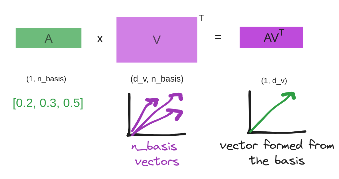
Attention read as a weighted sum over a basis of vectors $V$, with coefficients drawn from the attention matrix $A$.
The key point here is that our $A$ matrix attends to the different basis vectors, we’ll show how this can be chosen in a minute, but the key point here is that we have n basis vectors which we want a normalized vector of coefficients to have some understanding of.
Projection back to residual stream Note, however, this product $(n_{context} \times n_{basis}) \cdot (n_{basis} \times d_{v}) = (n_{context} \times d_{v})$ leaves the residual stream vector to be of size $d_v$. So finally if we want to add these vectors back to their to obtain a fuller description of such a way of propagation we want a matrix $W_O$ to project the propagated information back out:
$$h(x^l) = AV^TW_O^T$$Note for this reason, some sources use the notation of the above equalling $x^{l+2}$ instead. This is actually the full matrix product of the attention layer:
$$h(x^l) = A x^{l} W_V^TW_O^T = (A \otimes W_O W_V) \cdot x^l$$The attention scores matrix, $A$ The detail we’re missing here lies in how we parameterise $A$. We want $A$ to have the following property:
$$ \sum_{n=1}^{n_{basis}} a_{mn} = 1 $$This guarantees that when we weight our vectors, we are confined to getting a vector that is of the same order of magnitude as the basis $V$. This can be achieved by the following reparameterisation of $A$:
$$A=Softmax(W)$$Where the Softmax is applied across the basis vector dimension.
The remaining question is where $W$ comes from, and the answer is that each token proposes what it’s looking for and what it has to offer: $W = QK^T/\sqrt{d_k}$, with $Q = x^lW_Q^T$ and $K = x^lW_K^T$. The scaling keeps the Softmax out of its saturated regime. That gives the circuits form of a head as two separable products, $(A \otimes W_OW_V)$, where $A$ itself depends on $x^l$ through $W_QW_K$ — one circuit deciding where to read from, the other deciding what to write back.
Conclusion
Transformers get their efficiency from how nearly everything in them is matrix multiplication. There is very little else going on: stack the right products in the right order, and the only thing on the path we traced that isn’t linear is the Softmax normalising the attention scores.
The zero-layer transformer is, I think, the most useful thing to hold onto. Paired with the off-by-one input-output training, it gives a really clean picture of what the embedding and unembedding layers are natively trying to do: with no attention attached at all, $(I \otimes W_UW_E)$ is already learning what tends to follow what, token by token, with no notion of context.
Everything beyond that is machinery for letting tokens talk to one another. That turns out to be a case of forming a basis set of vectors from the query and key indices, taking their similarity, and using it to pull from a basis set formed from those same tokens — the value vectors.
Circuits notation then gives you an easy way to view and compose all of this. A head is $(A \otimes W_OW_V)$: one product across positions, one across features, and the two compose cleanly.
References
- Elhage, N., Nanda, N., Olsson, C., Henighan, T., Joseph, N., Mann, B., Askell, A., Bai, Y., Chen, A., Conerly, T., DasSarma, N., Drain, D., Ganguli, D., Hatfield-Dodds, Z., Hernandez, D., Jones, A., Kernion, J., Lovitt, L., Ndousse, K., Amodei, D., Brown, T., Clark, J., Kaplan, J., McCandlish, S., & Olah, C. (2021). A mathematical framework for Transformer circuits. Transformer Circuits Thread. https://transformer-circuits.pub/2021/framework/index.html